Image to light curve
Reviewable
Differential Photometry Mode
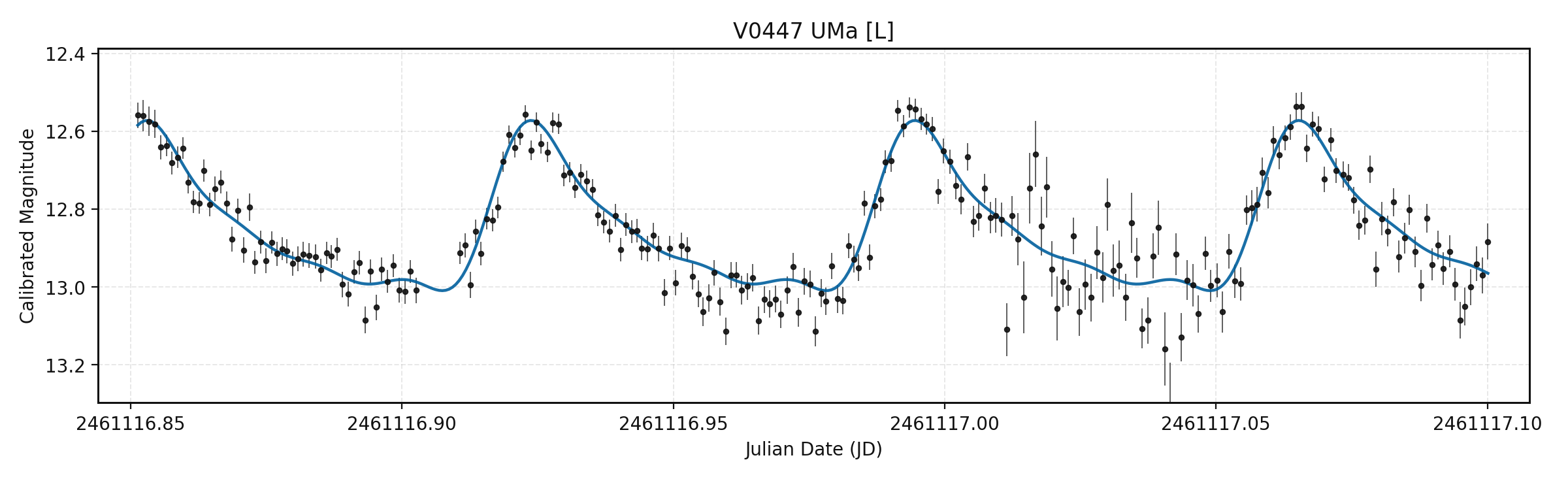
Open an image sequence. CAst finds all known variables and exoplanet hosts in the field, intelligently chooses comparison stars for each one, and measures their light curves within minutes.
What differential photometry reveals
A star can pulsate, rotate, eclipse a companion, or dim when a planet crosses it. Differential photometry measures that change against stable stars observed through the same atmosphere and optics.
Smart field-wide analysis
From solved field to complete light curves in minutes.
Identified across the field automatically.
Chosen separately for each target.
Generated for the whole field within minutes.
Automatic first. Scan Comps and fully manual apertures remain available when you need them. Differential Photometry is only one mode inside CAst.
From measurement to interpretation
The analysis tools stay beside the data, so a classroom demonstration and a scientific review can follow the same reduction.
Compare harmonic and Box Least Squares searches, fold repeated cycles, and inspect whether an eclipse or transit remains coherent.
Mark minima or maxima, import historical extrema, pull supported AAVSO data, and compare observed event times with an ephemeris.
Keep the target centered while a scanner moves over the light curve. Shared clouds and a true stellar event become easier to distinguish.
AAVSO-ready export
Select the targets and choose File → Export Report. CAst writes the AAVSO Extended Format file and checks observer code, chart ID, STD/DIF, filter, airmass, and skipped rows before export.
Free and open source
CAst is free, open source, and under regular development. Beginners can follow the guided workflow; experienced observers can inspect settings, intermediate measurements, exclusions, formulas, and provenance instead of accepting an unexplained curve.
Start the complete tutorialComplete tutorial
Follow the operating sequence first. Settings and calculations are kept in their own references so the instructions never jump away from the task in front of you.
The window title changes to Citizen Astronomy - Differential Photometry. The main action at the top left is Open.
Differential Photometry measures a time series of one field. HR Diagram mode measures many stars in one source image.
Use .fit, .fits, .xisf, .tif, .tiff, or a supported camera RAW format such as .cr2, .cr3, .nef, .arw, or .dng. JPG and PNG files are reported and ignored.
CAst warns before loading RAW files. If you continue, it decodes the color-camera data as linear 16-bit RGB and averages the demosaiced channels into one synthetic luminance plane. Bayer interpolation, camera color response, white balance, and star color can bias precise measurements. For scientific or AAVSO work, validate the result or preprocess the sequence into one calibrated, consistent channel first.
Capture Folder, Pipeline, Progress, Generate, and the object-selection table.
File → Open Folder also scans a folder. The top-left Open path is better for a first run because it keeps the options and progress together. Do not use File → Open File for a time series.
Use designation filters to choose catalog families. Brightest Variables limits a dense field by percentage. Analyze Best is an alternative field-screening path for strong measurable targets; it is not another percentage filter.
If the image timestamps omit a timezone, set Image Timestamp Timezone before Generate.
Generate scans metadata, validates WCS, queries field catalogs, builds target-specific comparison pools, estimates seeing, measures the images, creates magnitude contexts, applies quality analysis, and builds light curves.
Filter variables, checks, exoplanets, or references. Use Process Default for the configured limit, Process All Visible after filtering, or Process Selected for highlighted rows.
Show designation counts, source types, and the three process buttons.
After Generate, CAst normally selects Filter: Overview and Y: Standard Magnitude.
The gear beside Source Results opens Filter Source Results. There is no permanent name/type search row in the current layout.
Use Display, Curves, or Invert to make the field easier to see. These are preview controls and do not change measurement pixels.
Check saturation, SNR, centroid shift, comparison scatter, background, flux error, and the original frame. Use Overview to see whether comparisons and the check star contain the same trend.
Click Filter for Filtering Settings. Filtering changes the analysis/view; it does not delete the original measurement. Export Report preserves accepted and rejected rows separately.
An isolated point may be a bad frame, but it may also be ingress, egress, flare structure, or a real extremum. Inspect the image and comparison series first.
CAst starts with a target-specific ensemble ranked mainly by magnitude similarity and then separation.
The editor starts independently of the selected automatic target. Enable Keep Comparison Stars in Settings → Light Curve only when you want to seed the manual set from the automatic ensemble.
Click Increase SNR to combine adjacent measurements. CAst limits bins by variability type and period: 1.5% for sharp variables/transits, 5% for smooth variables, and 3% otherwise, with a default 600-second absolute cap.
The button changes to Reset SNR. Use it to restore the original cached series. In-bin outlier rejection is optional and off by default in Advanced settings.
Click Fold to compare repeated cycles at phase φ = ((t − t₀) / P) mod 1. A plausible period should align the event without creating the same structure in comparison/check stars.
C(E) = T₀ + EPO − C = Tobserved − C(E)A slope suggests the adopted epoch/period is offset. Curvature can motivate a period-change analysis, but it is not by itself proof of a physical mechanism.
Candidate score is triage, not a discovery claim. Check artifacts, catalogs, surveys, and additional nights. Label and Train Model build an optional local detectability classifier from your own labeled examples.
MTYPE=STD requires a valid standard-magnitude context; otherwise the row is DIF. TRANS=YES is written only for STD rows when you explicitly mark the data transformed. CAst does not calculate transformation coefficients.
Show Combined, Star Field, Light Curve, composition controls, and Export Animation.
Settings are grouped here so the operating steps remain continuous.
Set the astrometry.net API key and timeout when remote solving is needed. Embedded WCS and local Gaia matching can still work without a key.
Set Observer Code, observer/organization, fallback AAVSO filter, Sequence/Chart ID, optional API token, Image Timestamp Timezone, Transformed Data, and Reduction Notes. Set site latitude, longitude, and elevation under Setup for ephemeris and computed airmass.
WCS Sanity Check controls sample quality, approval, residual, isolation, coherent-shift, soft-accept, CCVALS repair, and Gaia magnitude limits. Increase SNR controls target SNR, period fractions, duration, frame count, weighting, and optional clipping. Change advanced values only with a repeatable reason from Work Log or the data.
Choose axes, fit mode, Infer method, phase behavior, grid, valid-only display, Keep Comparison Stars, equatorial grid, and recentering. These controls belong to review and presentation, so they are separate from the pipeline settings dialog.
Choose Aligned only when frames share pixel geometry. Refresh or clear catalog cache when a field query is demonstrably stale or incomplete.
Confirm the supported extension, timestamps, metadata, and selected folder. JPG and PNG are intentionally excluded. A camera RAW file must be readable by LibRaw.
Check the celestial solution and Work Log. Add an astrometry.net key when needed. Tune WCS sanity only after understanding the failed probe.
Check designation filters and preview limits, or rerun Select Sources To Process with Process All Visible.
Inspect Overview, clouds, tracking, gradients, and saturation. Use Scan Comps or create a manual ensemble with a check star.
Check filter naming and band-matched comparison catalog data. Differential Magnitude remains the relative measurement.
Clear the current folder or selected object when possible. File → Clear All Cache is the application-wide reset and keeps settings.
Advanced reference
This is the implemented calculation chain. It follows the pixels through calibration, apertures, comparison ensembles, quality analysis, period search, discovery scoring, and AAVSO export.
Naive observation timestamps use the configured timezone. The AAVSO timestamp is shifted to mid-exposure:
JDmid = JDstart + texp / (2 × 86400)Core differential times are UTC-derived JD. O-C imports may supply JD, HJD, or BJD; the reduction does not calculate a barycentric correction per frame.
Optional calibration applies:
Ical = (Ilight − Ibias − sIdark) / Iflat,norms = tlight / tdarkMasters are pixel medians. The corrected flat is normalized by its positive-pixel median; unsafe values become 1 and non-finite science pixels become 0.
CAst accepts coherent embedded WCS, repairs CRVAL from CCVALS when appropriate, or races local Gaia matching against astrometry.net when configured.
A 15 × 15 cutout is background-clipped at 3σ. The stellar core is kept above max(0.03 × peak, 1.5 × background scatter). CAst interpolates the half-maximum radius and uses FWHM = 2r½; second moments give FWHM = 2.35482σ as fallback.
rap = 1.6 FWHMrin = 3.0 FWHMrout = 4.5 FWHMThe 3σ-clipped annulus median is subtracted from the aperture:
F = Saperture − B̃ Aapertureminst = −2.5 log10(F)σF = √(|F| + nap σB² + nap² σB² / nsky)σm = (2.5 / ln 10)(σF / F)This source-plus-background propagation supplies current measurement errors and exported MERR. The codebase also contains tested full CCD, scintillation, and empirical-scatter routines, but they are not wired into PhotometryMeasurement or AAVSO MERR and are not claimed here as active.
Eligible comparisons are ranked per target by catalog-magnitude similarity, then distance. Stars within 30 arcsec of a known variable are excluded.
wi = 1 / σFi²Fref = Σ(wiFi) / ΣwiΔm = −2.5 log10(Ftarget / Fref)If useful flux errors are unavailable, reference flux falls back to an unweighted median.
σΔm = (2.5 / ln 10) √[(σFt / Ft)² + (σFr / Fr)²]ZPi = mcatalog,i − minst,imtarget = minst,target + ZPWhen every zero-point error is usable, ZP = Σ(ZPi / σi²) / Σ(1 / σi²). Otherwise CAst uses the arithmetic mean and, for multiple references, the standard error. Standard Magnitude seeks a band match from VSP/APASS and falls back toward Gaia when necessary.
SNR < 5: −0.18; SNR < 3: exclude.
Centroid shift > 2.5 px: −0.10; > 4 px: exclude.
Comparison scatter > 8%: −0.15; > 18%: exclude.
Global MAD or local Hampel z > 4.5: −0.28 and exclude.
Other soft flags: −0.05 each; score < 0.35: exclude.
Saturation or non-positive flux: hard exclusion.
σrobust = 1.4826 median(|x − median(x)|)z = |x − median(x)| / σrobustNear-saturation begins at 95% of the resolved threshold. Rejected points remain in the report with their reasons.
f(t) = a₀ + Σk[ak cos(2πkt/P) + bk sin(2πkt/P)]Harmonic Fit solves a Fourier series with up to six harmonics over 240 coarse logarithmic trial periods and three refinements. It tests 2P, 3P, and 4P and chooses by Bayesian Information Criterion. BLS uses a period/duration grid for box-shaped events.
The lower search bound is the larger of the configured minimum and twice median cadence. The upper bound is the smaller of the configured maximum and 95% of the time span. A result within 0.5% of either boundary is rejected.
nframes = ceil((SNRtarget / median SNR)²)C(E) = T₀ + EPO − C = Tobserved − C(E)Binning remains subject to period-fraction, duration, and frame-count caps. In-bin clipping is optional and off by default.
Discovery calculates RMS, MAD, 5th–95th percentile amplitude, reduced χ², von Neumann ratio, and Stetson J/K.
η = mean[(xi+1 − xi)²] / Var(x)δi = √(N / (N − 1)) (xi − mean(x)) / σiJ = mean[sign(δiδi+1) √|δiδi+1|]K = mean(|δ|) / √mean(δ²)The 0–100 score adds capped contributions: 30 min(log10χ²r / 1.4, 1), 20 min((MAD / σtyp) / 6, 1), 20 min((amplitude / σtyp) / 10, 1), 20 min(J / 4, 1) for positive J, and 10 min(max(0, 2 − η) / 1.5, 1). Stetson K is reported but is not a direct score term.
The optional classifier uses 160 trees with balanced-subsample class weighting after local labels exist.
Airmass is read from the header or estimated geometrically as X = sec(z) from the observing site. The Extended Format row records mid-exposure JD, magnitude/error, filter, STD/DIF, transformation flag, comparison/check metadata, airmass, chart, and notes.
For a cataloged check star, CAst reports rcheck = mcheck,cal − mcheck,catalog and the series RMS of those residuals. This diagnoses accuracy but is not added to each point's MERR.
CAst does not perform PSF deblending, derive color-transformation coefficients, model second-order extinction, apply a per-frame barycentric correction, or add scintillation/full CCD terms to the active MERR. Crowded fields and sub-millimagnitude work may require a different reduction.
Start with the data you have
Generate the first result automatically, inspect every assumption, and export only after the image, comparisons, curve, and metadata agree.